Setting up a workbook
Open Excel and create a blank workbook. The default settings will create three Worksheets, that’s enough. My personal settings only create one sheet, the others are inserted by ‘Insert->Worksheet’. For the beginning we need two sheets. These are renamed (rightclick on tab->Rename) to ‘budget’ and (for actual reasons) ‘2009’. Then go to ‘File->Save as…’ and save it.

renaming the tabs

Setting up the budget sheet
This first tutorial covers a rather simple approach, with month, account, several incomes and expenditures. I have chosen some examples for now.

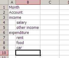
setting up the budget sheet

Just put Jan-2009 into C9, select C9 per simple click, grab the little lower-right-corner-square and drag it vertically to get the months filled in automatically.

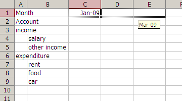
autofilling the months

Setting up the input sheet
For obvious reasons, ‘2009’ will be our input sheet. Four columns are enough for the moment.

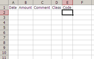
setting up the input sheet

‘Date’ is when, ‘Amount’ is how much and ‘Comment’ is your description what for you made the payment/got the money. The ‘Class’ will be necessary to get the numbers to the right place. Then there is ‘Code’. This cell is used for transferring payments to the budget sheet.
‘Class’ holds the payment types of the budget sheet. To get it a bit more comfortable, copy all of them to a free column of the input sheet. Then mark column D, ‘Data->Validation’, select ‘List’ and fill ‘Source’ with the range of your payment types. Click OK, do the same for D1 but this time select ‘Any Value’ to have a valid header. Now you can choose the class via drop down, this comes in handy when you handle more payment types.

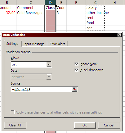
data validation for drop down menus

We’ll use the concatenate function in ‘Code’:

CONCATENATE(text1, text2,…) is used to join several text strings into a single string. The formula for E2 is:

=CONCATENATE(MONTH(A2), D2)

This will give us a string containing the number of the month and the payment classification. Some examples:

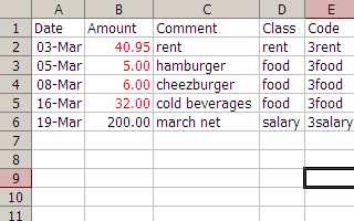
Code examples

Transferring inputs to the budget
Though it seems a lot of work, calm down, once it is set up, it’ll work forever. Err, through 2009. On the budget sheet ‘Account’, ‘income’ and ‘expenditure’ are simple sums (=sum(range)), I think you’ll get that. The interesting part is transferring the payments to their location. C4 therefore gets the following function:

=SUMIF(‘2009′!$E:$E,CONCATENATE(MONTH(C$1),$B4),’2009’!$B:$B)

SUMIF(range, criteria, sum_range) sums certain cells by given criteria. The range here is the ‘Code’ column in the input sheet, for the matching criteria the same concatenate procedure is used with the month row and the class column of the budget sheet. The sum_range obviously is the ‘Amount’ column. Be aware of the absolut references
indicated by ‘$’. This enables us to just fill the remaining cells in the budget sheet by dragging. It should instantly show results.

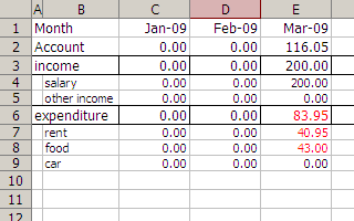
accounting

As this is a basic tutorial there will be no refining today. It just works!

Now count yer bluddy pieces o’ eight. Arrr!